What does this worked example show?

A real watershed segmentation of a coarse-sand photograph, run with the same algorithm as the live grain-size-distribution tool. 113 grains were detected; the resulting cumulative grain-size distribution gives D16 = 1.21 mm, D50 = 1.68 mm, D84 = 2.49 mm under an assumed 50 mm field of view.

Why is the field-of-view assumed?

The original photograph does not contain a scale reference (no coin, ruler, or card). Without that, every reported D-value is in pixel space. To produce numbers in millimeters for this example, we assume a 50 mm field-of-view — a typical close-up macro framing. In real use, always include a scale reference; the tool will refuse to compute mm-scale results otherwise.

What's the verbal interpretation of these numbers?

D50 = 1.68 mm sits in the very-coarse-sand class on the Wentworth scale (1–2 mm). The sample bridges coarse sand through granule. Folk-Ward σ = 0.54 φ classifies as moderately well sorted (Folk & Ward 1957). 54.9% of the area is very coarse sand and 38.1% is granule (2–4 mm), with a 7.0% coarse-sand tail. The distribution is unimodal.

Can I run this same analysis on my own photo?

Yes — open the live tool and either upload your photo or click "Load sample image" to pre-load the same coarse-sand photograph used here. Tap two endpoints of your scale object to calibrate, then click Analyze. Results render in 1–4 seconds for a typical phone photo.

← Back to the live tool Print with PE stamp box Designed for sealed engineering submittals — print drops PE stamp + signature block at the end.

Photo-Sieve Grain Size Distribution — Worked Example

A real watershed segmentation of a coarse-sand photograph using the PE-Calc photo-sieve calculator. Output: 113 individual grains, D₁₆ = 1.21 mm, D₅₀ = 1.68 mm, D₈₄ = 2.49 mm, Folk-Ward sorting σ = 0.54 φ (moderately well sorted). Static numbers and charts on this page; click through to the live tool to run the same analysis (or upload your own photo) end-to-end in your browser.

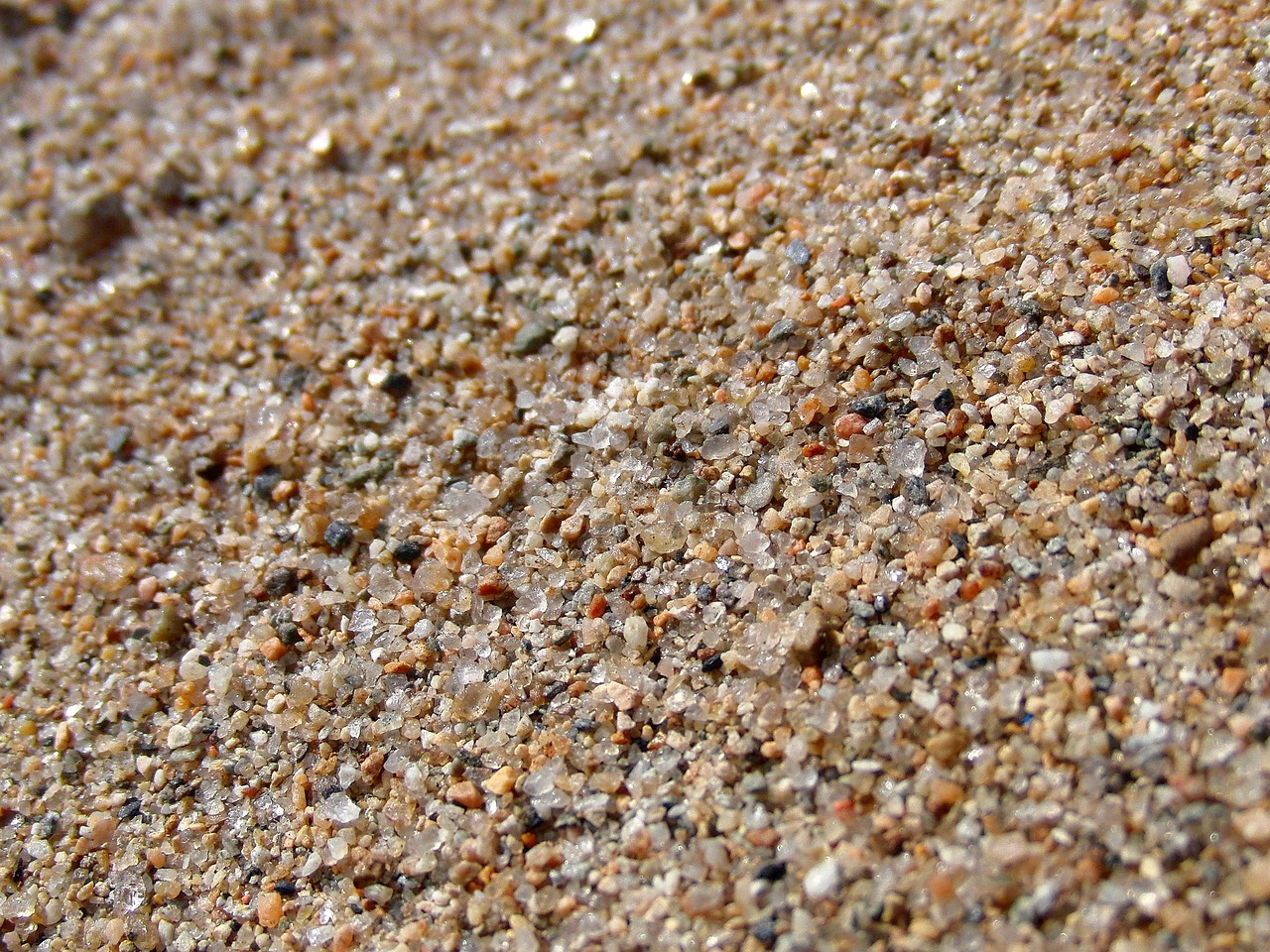
Input photograph

A 1280 × 960 macro photograph of beach / river sand. The image was selected because it contains a representative mix of coarse sand and granule-sized grains in a single layer with reasonable contrast between grains and inter-grain shadow. Note: the photograph contains no scale reference (no coin, ruler, or card). For the example we assume a 50 mm field-of-view across the long edge — typical for a phone-camera macro shot. Under that assumption the pixel scale is 25.6 px/mm, and every reported size carries that calibration uncertainty linearly.

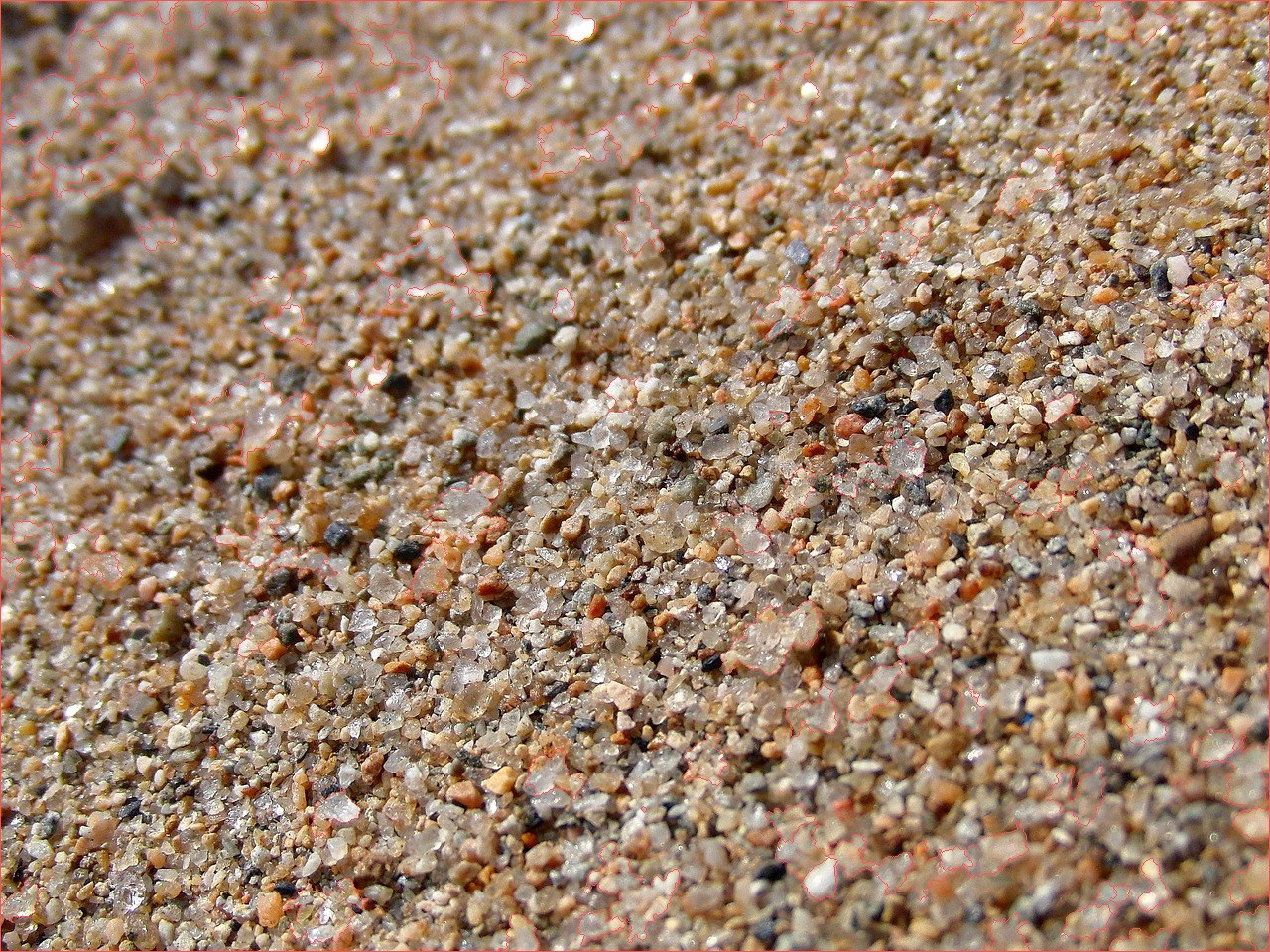
Coarse-sand and granule sample, 1280 × 960, top-down photograph used as the worked example — Source photograph — coarse sand and granules. 1280 × 960 px. Assumed field-of-view 50 mm.

Watershed segmentation overlay

Same image after the OpenCV.js pipeline: CLAHE local contrast → Otsu threshold → morphological cleanup → distance transform → marker-based watershed. The red lines are the watershed boundaries (label = −1 in the marker matrix). Each enclosed region is one grain whose b-axis is then measured by minimum-area bounding rectangle.

Distribution statistics

Grains

113

D₅

0.92 mm

D₁₆

1.21 mm

D₅₀ (median)

1.68 mm

D₈₄

2.49 mm

D₉₀

2.51 mm

D₉₅

3.30 mm

Mean (area-wt.)

1.83 mm

Sorting σ_I

0.54 φ

Verbal sorting

Moderately well

Total area

2.26 cm²

Wentworth class breakdown

Wentworth size class distribution — by grain area and by grain count
Class	Range (mm)	% area	% count	N
Silt / clay	< 0.0625	0.0	0.0	0
Very fine sand	0.0625 – 0.125	0.0	0.0	0
Fine sand	0.125 – 0.25	0.0	0.0	0
Medium sand	0.25 – 0.5	0.0	0.0	0
Coarse sand	0.5 – 1.0	7.0	20.4	23
Very coarse sand	1.0 – 2.0	54.9	61.9	70
Granule	2.0 – 4.0	38.1	17.7	20
Pebble	4 – 64	0.0	0.0	0

Reading the table: 54.9% of the total grain area falls in the very-coarse-sand class (1–2 mm). The 17.7% count vs. 38.1% area in the granule class is consistent: granule-sized grains are a minority by count but contribute disproportionately to total area because area scales with d². This count-vs-area split is the photographic equivalent of the count-vs-mass split in mechanical sieving.

Cumulative grain-size distribution

X-axis is the b-axis in millimeters on a log scale. Y-axis is cumulative percent finer by area. Orange dashed lines mark the standard percentiles read off the curve.

The S-curve is sigmoidal in log space — characteristic of a single-source unimodal sediment. The relatively short coarse and fine tails support the moderately-well-sorted classification.

Phi-scale histogram

X-axis is the phi unit, φ = −log₂(d_mm). Coarse grains plot at left (negative φ), fine grains at right (positive φ). Bin widths are 0.5 φ.

Mode at φ = −1 to 0 (1 to 2 mm). Tail toward fine end (positive φ) is short — consistent with a transport-sorted sample where finer fractions have been winnowed.

Step-by-step computation

Step 1 — Calibration

Input: assumed 50 mm field-of-view across the 1280-pixel long edge of the photograph.

px_per_mm = 1280 / 50 = 25.6 px/mm

All grain measurements below are in millimeters under this calibration.

Step 2 — Segmentation

Pipeline: CLAHE → Gaussian blur (5×5) → Otsu threshold → morphological open + close (3×3 kernel) → distance transform → threshold dist>0.45 for sure-foreground → 3-iteration dilation for sure-background → marker-based watershed.

Connected components on sure-foreground gives 121 raw markers.

After watershed, 113 candidate grains pass the filters: not touching image border, ≥10 pixels of area, <25% of total image area, b-axis ≥ 0.5 mm.

113 grains contribute to the distribution.

Step 3 — Per-grain b-axis

For each grain: fit a minimum-area bounding rectangle to the watershed contour. The shorter side is the b-axis. Convert pixels to mm using the calibration above.

Example: a grain whose minAreaRect is 28 × 41 px → b = 28 / 25.6 = 1.094 mm; area count of 720 px² → 720 / 25.6² = 1.099 mm² of grain area.

Step 4 — Area-weighted percentiles

Sort: grains by ascending b-axis; accumulate area; report the b-axis at which cumulative area crosses each target percentile.

Total grain area: 113 grains × ⟨area⟩ = 226.2 mm² = 2.26 cm².

D₅₀ = 1.68 mm: half the total area belongs to grains 1.68 mm or smaller.

D₁₆ = 1.21 mm and D₈₄ = 2.49 mm: the central 68% of the area lies between these two sizes.

Step 5 — Folk-Ward sorting

Convert to phi units: φ = −log₂(d_mm).

φ_{D5} = −log₂(0.92) = +0.13 · φ_{D16} = −log₂(1.21) = −0.27 · φ_{D84} = −log₂(2.49) = −1.32 · φ_{D95} = −log₂(3.30) = −1.72

σ_I = (φ_{D16} − φ_{D84}) / 4 + (φ_{D5} − φ_{D95}) / 6.6 = (−0.27 − (−1.32))/4 + (0.13 − (−1.72))/6.6

σ_I = 1.05/4 + 1.85/6.6 = 0.26 + 0.28

σ_I = 0.54 φ → "moderately well sorted" on the Folk-Ward verbal scale.

What this tells you

Wentworth call: the sample is dominantly very coarse sand (1–2 mm) with a notable granule fraction (2–4 mm). The coarse-sand tail is small. There is no measurable medium-sand or finer fraction in the visible top layer.
Sorting: moderately well sorted (σ_I ≈ 0.54 φ) is consistent with a transport-active environment — the photograph is plausibly a beach face, river bar, or eolian deposit where similar-sized grains have been segregated by repeated transport events.
Mean (1.83 mm) vs. median (1.68 mm): the area-weighted mean is slightly larger than the median, indicating a coarse-tail skew. The 38% granule fraction by area dominates the upper half of the distribution.
Caveat — the photograph has no scale. If the actual field-of-view were 30 mm (closer macro), all sizes would scale to 60% of these values: D₅₀ ≈ 1.0 mm (coarse sand). If 80 mm (wider framing), D₅₀ ≈ 2.7 mm (granule). Always include a scale reference in the field; this example demonstrates the method but its absolute values depend on the assumed calibration.

Run this analysis on your own photo

The live tool runs the exact same pipeline shown here. You can:

Open the live tool.
Click "Load sample image" to pre-load this same coarse-sand photograph (and the 50-mm-FOV custom calibration), then tap two endpoints to set the scale.
Or upload your own field photograph with a coin / ruler / credit card in frame for accurate calibration.

Apps for offline field use in development

Native iOS and Android apps with offline OpenCV are in development for high-throughput field surveys. Sign up to be notified at launch:

Coming soon App Store FieldHydro for iOS Coming soon Google Play FieldHydro for Android